Charnes, Cooper and Rhodes(3) recognised the difficulty in seeking a common set of weights to determine relative efficiency. They recognised the legitimacy of the proposal that units might value inputs and outputs differently and therefore adopt different weights, and proposed that each unit should be allowed to adopt a set of weights which shows it in the most favourable light in comparison to the other units. Under these circumstances, efficiency of a target unit j0 can be obtained as a solution to the following problem:
Maximise the efficiency of unit j0,
subject to the efficiency of all units being < =1.
The variables of the above problem are the weights and the solution produces the weights most favourable to unit j0 and also produces a measure of efficiency.
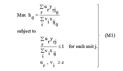
The algebraic model is as follows:
For the depot data, the efficiency of depot 1 is obtained by solving the following model:
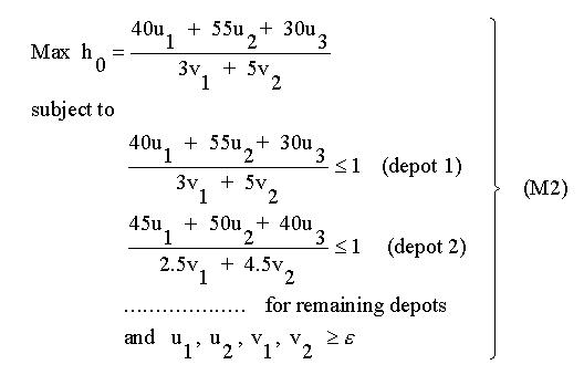
The u’s and v’s are variables of the problem and are constrained to be greater than or equal to some small positive quantity in order to avoid any input or output being totally ignored in determining the efficiency. The solution to the above model gives a value h0, the efficiency of depot 1, and the weights leading to that efficiency. If h0 = 1 then depot I is efficient relative to the others but if ho turns out to be less than l then some other depot(s) is more efficient than depot l, even when the weights are chosen to maximise depot l ‘s efficiency.
This flexibility in the choice of weights is both a weakness and a strength of this approach. It is a weakness because the judicious choice of weights by a unit possibly unrelated to the value of any input or output may allow a unit to appear efficient but there may be concern that this is more to do with the choice of weights than any inherent efficiency. This flexibility is also a strength, however, for if a unit turns out to be inefficient even when the most favourable weights have been incorporated in its efficiency measure then this is a strong statement and in particular the argument that the weights are incorrect is not tenable.
DEA thus may be appropriate where units can properly value inputs or outputs differently, or where there is a high uncertainty or disagreement over the value of some input or outputs.
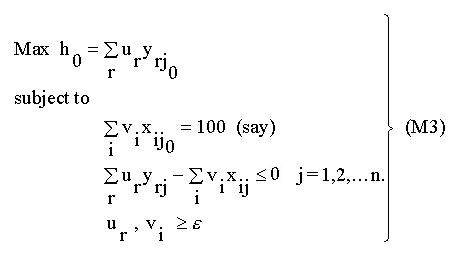
The DEA model M1 is a fractional linear program. To solve the model it is first necessary to convert-it into linear form so that the methods of linear programming can be applied. The linearisation process is relatively straightforward. The linear version of the constraints of Ml is shown in model M3. For the objective function it is necessary to observe that in maximising a fraction or ratio it is the relative magnitude of the numerator and denominator that are of interest and not their individual values. It is thus possible to achieve the same effect by setting the denominator equal to a constant and maximising the numerator. The resultant linear program is as follows: