Operational models

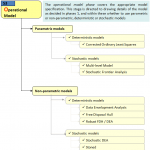
Dependant on (a) available data, (b) the quality of the data (e.g., noisy) and (c) the type of the data (e.g., negative values, discrete variables, desirable/undesirable values etc.), specific classes of models are available. Two main categories can be distinguished. As in Figure 5 the first class consists of parametric models (see, e.g., Greene, 2008). This family of models assumes an a priori specification on the production function (i.e., how the inputs are converted into outputs). The advantages of this procedure are its well established statistical inference and its easy inclusion of environmental characteristics. Its disadvantage lies in the a priori specification of the model. It is often very difficult to argue that the production process follows, e.g., a Cobb-Douglas, Translog or Fourier specification. The second class consists of the non-parametric models. They do not require any a priori assumptions on the production function. They therefore have more flexibility and, as such, let the data speak for themselves (Stolp, 1990). A disadvantage of this class lies in the restrictive curse of dimensionality and they often deliver a large variance and wide confidence interval.
Within these two families, both deterministic and stochastic variants exist. The deterministic models assume that all observations belong to the production set. This assumption makes them sensitive to outlying observations. However, robust models (Cazals et al., 2002) avoid this limitation. Stochastic models allow for noise in the data and capture the noise by an error term. However, sometimes it is difficult to distinguish the noise from inefficiency, the stochastic frontier models are specifically directed to this problem (Kumbhakar and Lovell, 2000).
The literature has developed several models for efficiency estimations (for an overview, Daraio and Simar, 2007). In the remainder of the paper, we will focus only on the non-parametric deterministic model. However, the researcher should be aware of the other model specifications, and even of particular variants of the traditional model specifications [e.g., Dula and Thrall (2001) developed a DEA model which is less computational demanding and, as such, interesting to analyze large datasets]. Although in the previous phase outliers and atypical observations were removed from the dataset (or at least inspected more carefully), the deterministic model is still vulnerable to these influential entities. To reduce the impact of outlying observations, Cazals et al. (2002) introduced robust efficiency measures. Instead of evaluating an entity against the full reference set, an entity is evaluated against a subset of size m. By taking the average of these evaluations, the estimates are less sensitive to outlying units. In addition, these so-called robust order-m efficiency estimates allow for statistical inference, such as standard deviations and confidence intervals.
Cazals et al. (2002) and Daraio and Simar (2005) developed conditional efficiency approach that include condition on exogenous characteristics in DEA models. This bridges the gap between parametric models (in which it is easy to include heterogeneity) and non-parametric models. Daraio and Simar (2007) develop conditional efficiency estimates for multivariate continuous variables. Badin et al. (2008) develop a data-driven bandwidth selection, while De Witte and Kortelainen (2008) extend the model to generalized discrete and continuous variables. By using robust conditional efficiency measures, many advantages of the parametric models are included now in the deterministic non-parametric models. Daraio and Simar (2007) present an adoption of the non-convex FDH and convex DEA efficiency scores to obtain conditional and robust framework.