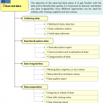
Having settled some preliminary questions in the first phase, in a second phase the researcher can start the analysis with the initial data collection. Especially in large datasets, it is worthwhile spending sufficient time with this phase (summarized in Figure 4). Various variables are potentially available and differences between them are sometimes subtle. In order to examine the research question from phase 1, additional data sources (such as statistical databases, annual accounts or price information) should have been consulted. This requires a sound method of data collection (in order to allow for reproduction of the dataset in the future). The latter is facilitated if a clear data collection routine is defined.
Having collected the data, it is necessary to characterize them at the meta level (i.e., describe and explore the data). The ‘explore data’ task typically consists of an initial report with summarisation and possibly visualisation of data. Although visualisation is limited to two or three dimensions, this frequently brings additional insights (Grinstein et al., 2002). Besides a brief description the ‘describe data task’ contains notification of the type of data (e.g., continuous or discrete) because different models can be adapted depending on the data type (Cook and Zhu, 2006).
Obviously, data can differ significantly in quality. Especially when compiling the data from different sources (e.g., two different types of hard data) or different data collection techniques (e.g., hard data combined with survey sample data) caution should be taken. For example, the definitions of the variables could differ according to the original source. But the quality of the combined dataset could be at stake in more subtle issues. For example, different data sources could have different random samples (so the data should be weighted accordingly: the researcher can account for this by, for example, (1) in the robust order-m estimations of Cazals et al. (2002) drawing less frequently observations from the minority group, or (2) in bootstrap replications, in comparison to the underrepresented observations, replicating fewer the overrepresented observations (for an empirical example, Cherchye et al., 2009). The researcher should be constantly aware of potential differences in data definitions and data collection techniques.
Depending on the applied assessment technique (MLM, COLS, FDH, DEA…; see phase 3) differences in data quality are increasing troublesome. Particularly in deterministic DEA models, outlying and atypical observations due to a low quality of data could heavily influence the outcomes. Fortunately, the non-parametric literature has developed several techniques to deal with, e.g., missing data (e.g., Kao and Liu, 2000), negative data (e.g., Emrouznejad et al., 2010a, 2010b and Portela et al., 2004), zero values (e.g., Thompson et al., 1993) or ratio data (Emrouznejad and Amin, 2009). Efficiency estimation with noisy data (e.g., due to measurement errors) could result in very imprecise results (for various models dealing with irregular data in DEA see Zhu and Cook; 2007). Therefore, it is worthwhile to examine the noise around the DEA estimates by bootstrapping techniques or statistical inferences (Simar and Wilson, 2007; see also phase 5).
In addition, observations with a dramatic impact on the efficiency scores of other observations could be removed from the sample. The literature developed several techniques to detect influential observations: the peer count index (Charnes et al., 1985), outlier detection by the use of super-efficiency model (Andersen and Petersen, 1993), order-m based models (Simar, 2003), leverage (Sousa and Stosic, 2005), etc. are typical techniques for non-parametric models. Outlier detection models exist for parametric models as well (e.g., Langford and Lewis, 1998 for MLM). Each of these models has its own peculiarities and, as such, it could be worthwhile to combine the different procedures (De Witte and Marques, 2010).
On the other hand, influential observations could be of increased interest as they could reveal extreme best practices or indicate where someone has specialized into a niche performance. Therefore, a researcher cannot simply remove the outliers from the sample (an alternative non-parametric approach which reduces the impact of outlying observations in the sample is the robust order-m model of Cazals et al., 2002; see phase 4). Finally, this sub-phase aims at obtaining a quality report on the data such that the weakest and strongest links can easily be noticed.
Once settled, the researcher has to prepare the final dataset on which the models will be run. The analyst has to collect the data from the different data sources, and deal with the missing, zero or negative data appropriately. Finally, he/she obtains a clean and ready to use dataset.


