For any linear program (LP) it is possible to formulate a partner LP using the same data, and the solution to either the original LP (the primal) or the partner (the dual) provides the same information about the problem being modelled. DEA is no exception to this.
The dual model is constructed by assigning a variable (dual variable) to each constraint in the primal model and constructing a new model on these variables. This is shown below.
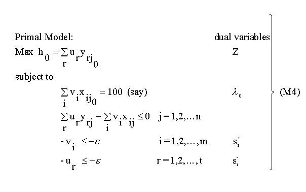
The first thing to note is that the primal model has n + t + m + 1 constraints whilst the dual model has m + t constraints. As n, the number of units, is usually considerably larger than t + m, the number of inputs and outputs, it can be seen that the primal model will have many more constraints than the dual model. For linear programs in general the more constraints the more difficult a problem is to solve. Hence for this reason it is usual to solve the dual DEA model rather than the primal.
From the theory of linear programming it is known that the values of the dual variables as a result of solving a dual model are identical to the shadow prices in the primal model. The dual variables Lambda(j) are thus also the shadow prices related to the constraints limiting the efficiency of each unit to be no greater than 1. It is also known that where a constraint is binding, a shadow price will be positive normally and where the constraint is non-binding the shadow price will be zero. In the solution to the primal model therefore a binding constraint implies that the corresponding unit has an efficiency of 1 and there will be a positive shadow price or dual variable. Hence positive shadow prices in the primal, or positive values for the Lambda(j) ‘s in the dual, correspond to and identify the peer group for any inefficient unit.
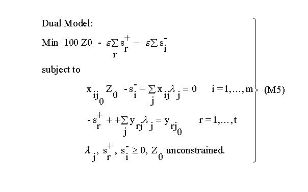
The dual model M5 can also be interpreted in terms of the composite unit introduced in the previous section. Rearranging M5 as M6 gives:
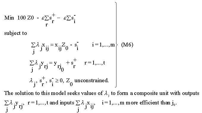
(Note that since the slack variables are non-negative and Z0 cannot exceed l, the composite unit has input levels that do not exceed those of unit j0 and output levels that are at least as high). If unit j0 is indeed efficient, the slacks will equal 0 and Z0 will equal 1, i.e. it has proved impossible to find a composite unit outperforming unit j0. If j0 is not efficient Z0 will be less than l and some slacks may be positive, i.e. it has proved possible to find a more efficient composite unit. The Lambda(j) ‘s form an efficient composite unit providing targets for j0, and Z0 represents the proportion of the input levels of j0 that the efficient composite unit would require to produce at least the output levels of j0. Z0 is thus a measure of the efficiency of j0. The composite unit thus provides a set of targets for an inefficient unit.